Coronagraph Basics
This set of exercises guides the user through a step-by-step process of simulating NIRCam coronagraphic observations of the HR 8799 exoplanetary system. The goal is to familiarize the user with basic pynrc classes and functions relevant to coronagraphy.
[1]:
# Import the usual libraries
import numpy as np
import matplotlib
import matplotlib.pyplot as plt

# Enable inline plotting at lower left
%matplotlib inline
We will start by first importing pynrc along with the obs_hci (High Contrast Imaging) class, which lives in the pynrc.obs_nircam module.
[2]:
import pynrc
from pynrc import nrc_utils          # Variety of useful functions and classes
from pynrc.obs_nircam import obs_hci # High-contrast imaging observation class

# Progress bar
from tqdm.auto import tqdm, trange

# Disable informational messages and only include warnings and higher
pynrc.setup_logging(level='WARN')
pyNRC log messages of level WARN and above will be shown.
pyNRC log outputs will be directed to the screen.
Source Definitions
The obs_hci class first requires two arguments describing the spectra of the science and reference sources (sp_sci and sp_ref, respectively. Each argument should be a Pysynphot spectrum already normalized to some known flux. pynrc includes built-in functions for generating spectra. The user may use either of these or should feel free to supply their own as long as it meets the requirements.
The
pynrc.stellar_spectrumfunction provides the simplest way to define a new spectrum:
bp_k = pynrc.bp_2mass('k') # Define bandpass to normalize spectrum
sp_sci = pynrc.stellar_spectrum('F0V', 5.24, 'vegamag', bp_k)
You can also be more specific about the stellar properties with Teff, metallicity, and log_g keywords.
sp_sci = pynrc.stellar_spectrum('F0V', 5.24, 'vegamag', bp_k,
                                Teff=7430, metallicity=-0.47, log_g=4.35)
Alternatively, the
pynrc.source_spectrumclass ingests spectral information of a given target and generates a model fit to the known photometric SED. Two model routines can be fit. The first is a very simple scale factor that is applied to the input spectrum, while the second takes the input spectrum and adds an IR excess modeled as a modified blackbody function. The user can find the relevant photometric data at http://vizier.u-strasbg.fr/vizier/sed/ and click download data as a VOTable.
[3]:
# Define 2MASS Ks bandpass and source information
bp_k = pynrc.bp_2mass('k')

# Science         source,  dist, age, sptype, Teff, [Fe/H], log_g, mag, band
args_sources = [('HR 8799', 39.0, 30,  'F0V', 7430, -0.47, 4.35, 5.24, bp_k)]

# References     source,     sptype, Teff, [Fe/H], log_g, mag, band
ref_sources = [('HD 220657', 'F8III', 5888, -0.01, 3.22, 3.04, bp_k)]
[4]:
name_sci, dist_sci, age, spt_sci, Teff_sci, feh_sci, logg_sci, mag_sci, bp_sci = args_sources[0]
name_ref, spt_ref, Teff_ref, feh_ref, logg_ref, mag_ref, bp_ref = ref_sources[0]

# For the purposes of simplicity, we will use pynrc.stellar_spectrum()
sp_sci = pynrc.stellar_spectrum(spt_sci, mag_sci, 'vegamag', bp_sci,
                                 Teff=Teff_sci, metallicity=feh_sci, log_g=logg_sci)
sp_sci.name = name_sci

# And the refernece source
sp_ref = pynrc.stellar_spectrum(spt_ref, mag_ref, 'vegamag', bp_ref,
                                 Teff=Teff_ref, metallicity=feh_ref, log_g=logg_ref)
sp_ref.name = name_ref
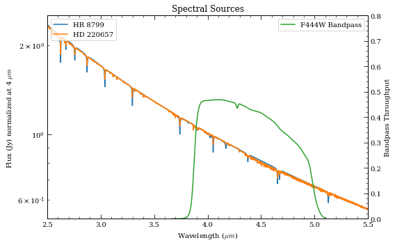
[5]:
# Plot the two spectra
fig, ax = plt.subplots(1,1, figsize=(8,5))

xr = [2.5,5.5]

for sp in [sp_sci, sp_ref]:
    w = sp.wave / 1e4
    ind = (w>=xr[0]) & (w<=xr[1])
    sp.convert('Jy')
    f = sp.flux / np.interp(4.0, w, sp.flux)
    ax.semilogy(w[ind], f[ind], lw=1.5, label=sp.name)
    ax.set_ylabel('Flux (Jy) normalized at 4 $\mu m$')
    sp.convert('flam')

ax.set_xlim(xr)
ax.set_xlabel(r'Wavelength ($\mu m$)')
ax.set_title('Spectral Sources')

# Overplot Filter Bandpass
bp = pynrc.read_filter('F444W', 'CIRCLYOT', 'MASK430R')
ax2 = ax.twinx()
ax2.plot(bp.wave/1e4, bp.throughput, color='C2', label=bp.name+' Bandpass')
ax2.set_ylim([0,0.8])
ax2.set_xlim(xr)
ax2.set_ylabel('Bandpass Throughput')

ax.legend(loc='upper left')
ax2.legend(loc='upper right')

fig.tight_layout()
Initialize Observation
Now we will initialize the high-contrast imaging class pynrc.obs_hci using the spectral objects and various other settings. The obs_hci object is a subclass of the more generalized NIRCam class. It implements new settings and functions specific to high-contrast imaging observations for corongraphy and direct imaging.
For this tutorial, we want to observe these targets using the MASK430R coronagraph in the F444W filter. All circular coronagraphic masks such as the 430R (R=round) should be paired with the CIRCLYOT pupil element, whereas wedge/bar masks are paired with WEDGELYOT pupil. Observations in the LW channel are most commonly observed in WINDOW mode with a 320x320 detector subarray size. Full detector sizes are also available.
The PSF simulation size (fov_pix keyword) should also be of similar size as the subarray window (recommend avoiding anything above fov_pix=1024 due to computation time and memory usage). Use odd numbers to center the PSF in the middle of the pixel. If fov_pix is specified as even, then PSFs get centered at the corners. This distinction really only matter for unocculted observations, (ie., where the PSF flux is concentrated in a tight central core).
The obs_hci class also allows one to specify WFE drift values in terms of nm RMS. The wfe_ref_drift parameter defaults to 2nm between
We also need to specify a WFE drift value (wfe_ref_drift parameter), which defines the anticipated drift in nm between the science and reference sources. For the moment, let’s intialize with a value of 0nm. This prevents an initially long process by which pynrc calculates changes made to the PSF over a wide range of drift values. This process only happens once, then stores the resulting coefficient residuals to disk for future quick retrieval.
Extended disk models can also be specified upon initialization using the disk_params keyword (which should be a dictionary).
The large_grid keyword controls the quality of PSF variations near and under the corongraphic masks. If False, then a sparse grid is used (faster to generate during initial calculations; less disk space and memory). If True, then a higher density grid is calculated (~2.5 hrs for initial creation; ~3.5x larger sizes), which produces improved PSFs at the SGD positions. For purposes of this demo, we set it to False.
[6]:
# The initial call make take some time, as it will need to generate coefficients
# to calculate PSF variations across wavelength, WFE drift, and mask location
filt, mask, pupil = ('F444W',  'MASK430R', 'CIRCLYOT')
wind_mode, subsize = ('WINDOW', 320)
fov_pix, oversample = (321, 2)

obs = pynrc.obs_hci(sp_sci, dist_sci, sp_ref=sp_ref, use_ap_info=False,
                    filter=filt, image_mask=mask, pupil_mask=pupil,
                    wind_mode=wind_mode, xpix=subsize, ypix=subsize,
                    fov_pix=fov_pix, oversample=oversample, large_grid=True)
Some information for the reference observation is stored in the attribute obs.Detector_ref, which is a separate NIRCam DetectorOps class that we use to keep track of the detector a multiaccum configurations, which may differe between science and reference observations. Settings for the reference observation can be updated using the obs.gen_ref() function.
[7]:
# Set default WFE drift values between Roll1, Roll2, and Ref

# WFE drift amount between rolls
obs.wfe_roll_drift = 2

# Drift amount between Roll 1 and Reference.
obs.wfe_ref_drift = 5
Exposure Settings
Optimization of exposure settings are demonstrated in another tutorial, so we will not repeat that process here. We can assume the optimization process was performed elsewhere to choose the DEEP8 pattern with 16 groups and 5 total integrations. These settings apply to each roll position of the science observation sequence as well as the for the reference observation.
[8]:
# Update both the science and reference observations
obs.update_detectors(read_mode='DEEP8', ngroup=16, nint=5, verbose=True)
obs.gen_ref_det(read_mode='DEEP8', ngroup=16, nint=5)
New Ramp Settings
  read_mode  :    DEEP8
  nf         :        8
  nd2        :       12
  ngroup     :       16
  nint       :        5
New Detector Settings
  wind_mode  :   WINDOW
  xpix       :      320
  ypix       :      320
  x0         :      914
  y0         :     1512
New Ramp Times
  t_group    :   21.381
  t_frame    :    1.069
  t_int      :  329.264
  t_int_tot1 :  330.353
  t_int_tot2 :  330.353
  t_exp      : 1646.322
  t_acq      : 1651.766
Add Planets
There are four known giant planets orbiting HR 8799. Ideally, we would like to position them at their predicted locations on the anticipated observation date. For this case, we choose a plausible observation date of November 1, 2022. To convert between \((x,y)\) and \((r,\theta)\), use the nrc_utils.xy_to_rtheta and nrc_utils.rtheta_to_xy functions.
When adding the planets, it doesn’t matter too much which exoplanet model spectrum we decide to use since the spectra are still fairly unconstrained at these wavelengths. We do know roughly the planets’ luminosities, so we can simply choose some reasonable model and renormalize it to the appropriate filter brightness.
Their are a few exoplanet models available to pynrc (SB12, BEX, COND), but let’s choose those from Spiegel & Burrows (2012).
[9]:
# Projected locations for date 11/01/2022
# These are prelimary positions, but within constrained orbital parameters
loc_list = [(-1.625, 0.564), (0.319, 0.886), (0.588, -0.384), (0.249, 0.294)]

# Estimated magnitudes within F444W filter
pmags = [16.0, 15.0, 14.6, 14.7]
[10]:
# Add planet information to observation class.
# These are stored in obs.planets.
# Can be cleared using obs.delete_planets().
obs.delete_planets()
for i, loc in enumerate(loc_list):
    obs.add_planet(model='SB12', mass=10, entropy=13, age=age, xy=loc, runits='arcsec',
                   renorm_args=(pmags[i], 'vegamag', obs.bandpass))
[11]:
# Generate and plot a noiseless slope image to verify orientation
PA1 = 85            # Telescope V3 PA
PA_offset = -1*PA1  # Image field is rotated opposite direction
im_planets = obs.gen_planets_image(PA_offset=PA_offset, return_oversample=False)
[12]:
from matplotlib.patches import Circle
from pynrc.nrc_utils import plotAxes
from pynrc.obs_nircam import get_cen_offsets

fig, ax = plt.subplots(figsize=(6,6))

xasec = obs.det_info['xpix'] * obs.pixelscale
yasec = obs.det_info['ypix'] * obs.pixelscale
extent = [-xasec/2, xasec/2, -yasec/2, yasec/2]
xylim = 4

vmin = 0
vmax = 0.5*im_planets.max()
ax.imshow(im_planets, extent=extent, vmin=vmin, vmax=vmax)

# Overlay the coronagraphic mask
detid = obs.Detector.detid
im_mask = obs.mask_images['DETSAMP']
# Do some masked transparency overlays
masked = np.ma.masked_where(im_mask>0.98*im_mask.max(), im_mask)
ax.imshow(1-masked, extent=extent, alpha=0.3, cmap='Greys_r', vmin=-0.5)

for loc in loc_list:
    xc, yc = get_cen_offsets(obs, idl_offset=loc, PA_offset=PA_offset)
    circle = Circle((xc,yc), radius=xylim/20., alpha=0.7, lw=1, edgecolor='red', facecolor='none')
    ax.add_artist(circle)

xlim = ylim = np.array([-1,1])*xylim
xlim = xlim + obs.bar_offset
ax.set_xlim(xlim)
ax.set_ylim(ylim)

ax.set_xlabel('Arcsec')
ax.set_ylabel('Arcsec')

ax.set_title('{} planets -- {} {}'.format(sp_sci.name, obs.filter, obs.image_mask))

color = 'grey'
ax.tick_params(axis='both', color=color, which='both')
for k in ax.spines.keys():
    ax.spines[k].set_color(color)

plotAxes(ax, width=1, headwidth=5, alength=0.15, angle=PA_offset,
                   position=(0.1,0.1), label1='E', label2='N')

fig.tight_layout()
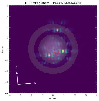
As we can see, even with “perfect PSF subtraction” and no noise, it’s difficult to make out planet e despite providing a similiar magnitude as d. This is primarily due to its location relative to the occulting mask reducing throughput along with confusion of bright diffraction spots from the other nearby sources.
Note: the circled regions of the expected planet positions don’t perfectly align with the PSFs, because the LW wavelengths have a slight dispersion through the Lyot mask material.
Estimated Performance
Now we are ready to determine contrast performance and sensitivites as a function of distance from the star.
1. Roll-Subtracted Images
First, we will create a quick simulated roll-subtracted image using the in gen_roll_image method. For the selected observation date of 11/1/2022, APT shows a PA range of 84\(^{\circ}\) to 96\(^{\circ}\). So, we’ll assume Roll 1 has PA1=85, while Roll 2 has PA2=95. In this case, “roll subtraction” simply creates two science images observed at different parallactic angles, then subtracts the same reference observation from each. The two results are then de-rotated to a common PA=0
and averaged.
There is also the option to create ADI images, where the other roll position becomes the reference star by setting no_ref=True.
Images generated with the gen_roll_image method will also include random pointing offsets described in the pointing_info dictionary. These can be generated by calling obs.gen_pointing_offsets().
[20]:
# Create pointing offset with a random seed for reproducibility
obs.gen_pointing_offsets(rand_seed=1234, verbose=True)
Pointing Info
  sgd_type   : None
  slew_std   : 5
  fsm_std    : None
  roll1      : [0.00370446 0.0007631 ]
  roll2      : [0.00431872 0.0145655 ]
  ref        : [-0.00801918  0.0003205 ]
[21]:
# Cycle through a few WFE drift values
wfe_list = [0,5,10]

# PA values for each roll
PA1, PA2 = (85,95)

# A dictionary of HDULists
hdul_dict = {}
for wfe_drift in tqdm(wfe_list):
    # Assume drift between Roll1 and Roll2 is 2 nm WFE
    wfe_roll_drift = 0 if wfe_drift<2 else 2
    hdulist = obs.gen_roll_image(PA1=PA1, PA2=PA2,
                                 wfe_ref_drift=wfe_drift, wfe_roll_drift=wfe_roll_drift)
    hdul_dict[wfe_drift] = hdulist
[22]:
from pynrc.nb_funcs import plot_hdulist
from matplotlib.patches import Circle

fig, axes = plt.subplots(1,3, figsize=(14,4.3))
xylim = 2.5
xlim = ylim = np.array([-1,1])*xylim

for j, wfe_drift in enumerate(wfe_list):
    ax = axes[j]
    hdul = hdul_dict[wfe_drift]

    plot_hdulist(hdul, xr=xlim, yr=ylim, ax=ax, vmin=0, vmax=10)

    # Location of planet
    for loc in loc_list:
        circle = Circle(loc, radius=xylim/15., lw=1, edgecolor='red', facecolor='none')
        ax.add_artist(circle)

    ax.set_title('$\Delta$WFE = {:.0f} nm'.format(wfe_drift))

    nrc_utils.plotAxes(ax, width=1, headwidth=5, alength=0.15, position=(0.9,0.1), label1='E', label2='N')

fig.suptitle('{} -- {} {}'.format(name_sci, obs.filter, obs.image_mask), fontsize=14)
fig.tight_layout()
fig.subplots_adjust(top=0.85)
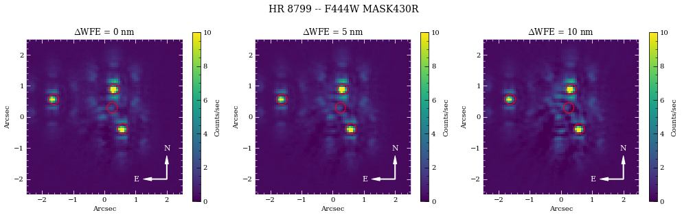
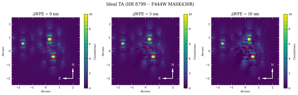
The majority of the speckle noise here originates from small pointing offsets between the roll positions and reference observation. These PSF centering mismatches dominate the subtraction residuals compared to the WFE drift variations. Small-grid dithers acquired during the reference observations should produce improved subtraction performance through PCA/KLIP algorithms. To get a better idea of the post-processing performance, we re-run these observations assuming perfect target acquisition.
[23]:
hdul_dict = {}
for wfe_drift in tqdm(wfe_list):
    # Assume drift between Roll1 and Roll2 is 2 nm WFE
    wfe_roll_drift = 0 if wfe_drift<2 else 2
    # Assume perfect centering by setting xyoff_***=(0,0)
    hdulist = obs.gen_roll_image(PA1=PA1, PA2=PA2,
                                 wfe_ref_drift=wfe_drift, wfe_roll_drift=wfe_roll_drift,
                                 xyoff_roll1=(0,0), xyoff_roll2=(0,0), xyoff_ref=(0,0))
    hdul_dict[wfe_drift] = hdulist
[24]:
from pynrc.nb_funcs import plot_hdulist
from matplotlib.patches import Circle

fig, axes = plt.subplots(1,3, figsize=(14,4.3))
xylim = 2.5
xlim = ylim = np.array([-1,1])*xylim

for j, wfe_drift in enumerate(wfe_list):
    ax = axes[j]
    hdul = hdul_dict[wfe_drift]

    plot_hdulist(hdul, xr=xlim, yr=ylim, ax=ax, vmin=0, vmax=10)

    # Location of planet
    for loc in loc_list:
        circle = Circle(loc, radius=xylim/15., lw=1, edgecolor='red', facecolor='none')
        ax.add_artist(circle)

    ax.set_title('$\Delta$WFE = {:.0f} nm'.format(wfe_drift))

    nrc_utils.plotAxes(ax, width=1, headwidth=5, alength=0.15, position=(0.9,0.1), label1='E', label2='N')

fig.suptitle('Ideal TA ({} -- {} {})'.format(name_sci, obs.filter, obs.image_mask), fontsize=14)
fig.tight_layout()
fig.subplots_adjust(top=0.85)
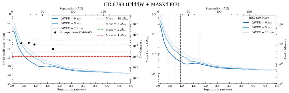
2. Contrast Curves
Next, we will cycle through a few WFE drift values to get an idea of potential predicted sensitivity curves. The calc_contrast method returns a tuple of three arrays:
The radius in arcsec.
The n-sigma contrast.
The n-sigma magnitude sensitivity limit (vega mag).
In order to better understand the relative contributes of WFE drift to contrast loss, we’re going to ignore telescope pointing offsets by explicitly passing xoff_* = (0,0) keywords for Roll 1, Roll 2, and Ref observations.
[25]:
nsig = 5
roll_angle = np.abs(PA2 - PA1)

curves = []
for wfe_drift in tqdm(wfe_list):
    # Assume drift between Roll1 and Roll2 is 2 nm WFE
    wfe_roll_drift = 0 if wfe_drift<2 else 2

    # Generate contrast curves
    result = obs.calc_contrast(roll_angle=roll_angle, nsig=nsig,
                               wfe_ref_drift=wfe_drift, wfe_roll_drift=wfe_roll_drift,
                               xyoff_roll1=(0,0), xyoff_roll2=(0,0), xyoff_ref=(0,0))
    curves.append(result)
[26]:
from pynrc.nb_funcs import plot_contrasts, plot_planet_patches, plot_contrasts_mjup, update_yscale
import matplotlib.patches as mpatches

# fig, ax = plt.subplots(figsize=(8,5))
fig, axes = plt.subplots(1,2, figsize=(14,4.5))
xr=[0,5]
yr=[24,8]

# 1a. Plot contrast curves and set x/y limits
ax = axes[0]
ax, ax2, ax3 = plot_contrasts(curves, nsig, wfe_list, obs=obs,
                              xr=xr, yr=yr, ax=ax, return_axes=True)
# 1b. Plot the locations of exoplanet companions
label = 'Companions ({})'.format(filt)
planet_dist = [np.sqrt(x**2+y**2) for x,y in loc_list]
ax.plot(planet_dist, pmags, marker='o', ls='None', label=label, color='k', zorder=10)

# 1c. Plot Spiegel & Burrows (2012) exoplanet fluxes (Hot Start)
plot_planet_patches(ax, obs, age=age, entropy=13, av_vals=None)
ax.legend(ncol=2)

# 2. Plot in terms of MJup using COND models
ax = axes[1]
ax1, ax2, ax3 = plot_contrasts_mjup(curves, nsig, wfe_list, obs=obs, age=age,
                                    ax=ax, twin_ax=True, xr=xr, yr=None, return_axes=True)
yr = [0.03,100]
for xval in planet_dist:
    ax.plot([xval,xval],yr, lw=1, ls='--', color='k', alpha=0.7)
update_yscale(ax1, 'log', ylim=yr)
yr_temp = np.array(ax1.get_ylim()) * 318.0
update_yscale(ax2, 'log', ylim=yr_temp)
# ax.set_yscale('log')
# ax.set_ylim([0.08,100])
ax.legend(loc='upper right', title='BEX ({:.0f} Myr)'.format(age))

fig.suptitle('{} ({} + {})'.format(name_sci, obs.filter, obs.image_mask), fontsize=16)

fig.tight_layout()
fig.subplots_adjust(top=0.85, bottom=0.1 , left=0.05, right=0.97)
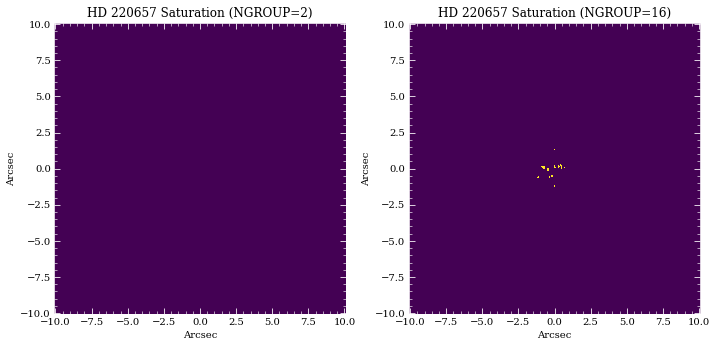
3. Saturation Levels
Create an image showing level of saturation for each pixel. For NIRCam, saturation is important to track for purposes of accurate slope fits and persistence correction. In this case, we will plot the saturation levels both at NGROUP=2 and NGROUP=obs.det_info['ngroup']. Saturation is defined at 80% well level, but can be modified using the well_frac keyword.
We want to perform this analysis for both science and reference targets.
[27]:
# Saturation limits
ng_max = obs.det_info['ngroup']
sp_flat = pynrc.stellar_spectrum('flat')

print('NGROUP=2')
_ = obs.sat_limits(sp=sp_flat,ngroup=2,verbose=True)

print('')
print(f'NGROUP={ng_max}')
_ = obs.sat_limits(sp=sp_flat,ngroup=ng_max,verbose=True)

mag_sci = obs.star_flux('vegamag')
mag_ref = obs.star_flux('vegamag', sp=obs.sp_ref)
print('')
print(f'{obs.sp_sci.name} flux at {obs.filter}: {mag_sci:0.2f} mags')
print(f'{obs.sp_ref.name} flux at {obs.filter}: {mag_ref:0.2f} mags')
NGROUP=2
F444W Saturation Limit assuming Flat spectrum in photlam source (point source): 1.29 vegamag
F444W Saturation Limit assuming Flat spectrum in photlam source (extended): 10.33 vegamag/arcsec^2

NGROUP=16
F444W Saturation Limit assuming Flat spectrum in photlam source (point source): 3.89 vegamag
F444W Saturation Limit assuming Flat spectrum in photlam source (extended): 12.93 vegamag/arcsec^2

HR 8799 flux at F444W: 5.24 mags
HD 220657 flux at F444W: 3.03 mags
In this case, we don’t expect HR 8799 to saturate. However, the reference source should have some saturated pixels before the end of an integration.
[28]:
# Well level of each pixel for science source
sci_levels1 = obs.saturation_levels(ngroup=2, exclude_planets=True)
sci_levels2 = obs.saturation_levels(ngroup=ng_max, exclude_planets=True)

# Which pixels are saturated? Assume sat level at 90% full well.
sci_mask1 = sci_levels1 > 0.9
sci_mask2 = sci_levels2 > 0.9
[29]:
# Well level of each pixel for reference source
ref_levels1 = obs.saturation_levels(ngroup=2, do_ref=True)
ref_levels2 = obs.saturation_levels(ngroup=ng_max, do_ref=True)

# Which pixels are saturated? Assume sat level at 90% full well.
ref_mask1 = ref_levels1 > 0.9
ref_mask2 = ref_levels2 > 0.9
[30]:
# How many saturated pixels?
nsat1_sci = len(sci_levels1[sci_mask1])
nsat2_sci = len(sci_levels2[sci_mask2])

print(obs.sp_sci.name)
print('{} saturated pixel at NGROUP=2'.format(nsat1_sci))
print('{} saturated pixel at NGROUP={}'.format(nsat2_sci,ng_max))

# How many saturated pixels?
nsat1_ref = len(ref_levels1[ref_mask1])
nsat2_ref = len(ref_levels2[ref_mask2])

print('')
print(obs.sp_ref.name)
print('{} saturated pixel at NGROUP=2'.format(nsat1_ref))
print('{} saturated pixel at NGROUP={}'.format(nsat2_ref,ng_max))
HR 8799
0 saturated pixel at NGROUP=2
0 saturated pixel at NGROUP=16

HD 220657
0 saturated pixel at NGROUP=2
44 saturated pixel at NGROUP=16
[31]:
# Saturation Mask for science target

nsat1, nsat2 = (nsat1_sci, nsat2_sci)
sat_mask1, sat_mask2 = (sci_mask1, sci_mask2)
sp = obs.sp_sci

# Only display saturation masks if there are saturated pixels
if nsat2 > 0:
    fig, axes = plt.subplots(1,2, figsize=(10,5))

    xasec = obs.det_info['xpix'] * obs.pixelscale
    yasec = obs.det_info['ypix'] * obs.pixelscale
    extent = [-xasec/2, xasec/2, -yasec/2, yasec/2]

    axes[0].imshow(sat_mask1, extent=extent)
    axes[1].imshow(sat_mask2, extent=extent)

    axes[0].set_title('{} Saturation (NGROUP=2)'.format(sp.name))
    axes[1].set_title('{} Saturation (NGROUP={})'.format(sp.name,ng_max))

    for ax in axes:
        ax.set_xlabel('Arcsec')
        ax.set_ylabel('Arcsec')

        ax.tick_params(axis='both', color='white', which='both')
        for k in ax.spines.keys():
            ax.spines[k].set_color('white')

    fig.tight_layout()
else:
    print('No saturation detected.')
No saturation detected.
[32]:
# Saturation Mask for reference

nsat1, nsat2 = (nsat1_ref, nsat2_ref)
sat_mask1, sat_mask2 = (ref_mask1, ref_mask2)
sp = obs.sp_ref

# Only display saturation masks if there are saturated pixels
if nsat2 > 0:
    fig, axes = plt.subplots(1,2, figsize=(10,5))

    xasec = obs.det_info['xpix'] * obs.pixelscale
    yasec = obs.det_info['ypix'] * obs.pixelscale
    extent = [-xasec/2, xasec/2, -yasec/2, yasec/2]

    axes[0].imshow(sat_mask1, extent=extent)
    axes[1].imshow(sat_mask2, extent=extent)

    axes[0].set_title(f'{sp.name} Saturation (NGROUP=2)')
    axes[1].set_title(f'{sp.name} Saturation (NGROUP={ng_max})')

    for ax in axes:
        ax.set_xlabel('Arcsec')
        ax.set_ylabel('Arcsec')

        ax.tick_params(axis='both', color='white', which='both')
        for k in ax.spines.keys():
            ax.spines[k].set_color('white')

    fig.tight_layout()
else:
    print('No saturation detected.')
[ ]: