Basic Usage
This tutorial walks through the basic usage of the pynrc package to calculate sensitivities and saturation limits for NIRCam in a variety of modes.
[1]:
# Import the usual libraries
import numpy as np
import matplotlib
import matplotlib.pyplot as plt

# Enable inline plotting at lower left
%matplotlib inline
Getting Started
We assume you have already installed pynrc as outlined in the documentation.
[2]:
# import main module
import pynrc
from pynrc import nrc_utils
Log messages for pynrc follow the same the logging functionality included in webbpsf. Logging levels include DEBUG, INFO, WARN, and ERROR.
[3]:
pynrc.setup_logging()
pyNRC log messages of level INFO and above will be shown.
pyNRC log outputs will be directed to the screen.
If you get tired of the INFO level messages, simply type:
pynrc.setup_logging('WARN', verbose=False)
First NIRCam Observation
The basic NIRCam object consists of all the instrument settings one would specify for a JWST observation, including filter, pupil, and coronagraphic mask selections along with detector subarray settings and ramp sampling cadence (i.e., MULTIACCUM).
The NIRCam class makes use of high order polynomial coefficient maps to quickly generate large numbers of monochromatic PSFs that can be convolved with arbitrary spectra and collapsed into a final broadband PSF (or dispersed with NIRCam’s slitless grisms). The PSF coefficients are calculated from a series of WebbPSF monochromatic PSFs and saved to disk. These polynomial coefficients are further modifed based on focal plane position and drift in the wavefront error relative to nominal OPD mao.
There are a multitude of posssible keywords one can pass upon initialization, including certain detector settings and PSF generation parameters. If not passed initially, then defaults are assumed. The user can update these parameters at any time by either setting attributes directly (e.g., filter, mask, pupil, etc.) along with using the update_detectors() and update_psf_coeff() methods.
For instance,
nrc = pynrc.NIRCam('F210M')
nrc.module = 'B'
nrc.update_detectors(read_mode='DEEP8', nint=10, ngroup=5)
is the same as:
nrc = pynrc.NIRCam('F210M', module='B', read_mode='DEEP8', nint=10, ngroup=5)
To start, we’ll set up a simple observation using the F430M filter. Defaults will be populated for unspecified attributes such as module, pupil, mask, etc.
Check the function docstrings for more detailed information
[4]:
nrc = pynrc.NIRCam(filter='F430M', fov_pix=33, oversample=4)
print(f'\nFilter: {nrc.filter};  Pupil Mask: {nrc.pupil_mask};  Image Mask: {nrc.image_mask};  Module: {nrc.module}')
[     stpsf:INFO] NIRCam aperture name updated to NRCA1_FULL
[     stpsf:INFO] NIRCam pixel scale switched to 0.062907 arcsec/pixel for the long wave channel.
[     stpsf:INFO] NIRCam aperture name updated to NRCA5_FULL
[     pynrc:INFO] RAPID readout mode selected.
[     pynrc:INFO] Setting ngroup=1, nf=1, nd1=0, nd2=0, nd3=0.
[     pynrc:INFO] Initializing SCA 485/A5
[     pynrc:INFO] Suggested SIAF aperture name: NRCA5_FULL
[     pynrc:INFO] RAPID readout mode selected.
[     pynrc:INFO] Setting ngroup=1, nf=1, nd1=0, nd2=0, nd3=0.
[     pynrc:INFO] Initializing SCA 485/A5
[webbpsf_ext:INFO] Loading /Users/jarron/NIRCam/webbpsf_ext_data/psf_coeffs/NIRCam/LWA_F430M_CLEAR_NONE_pix33_os4_jsig1_r0.00_th+0.0_OPD-2022-07-30_siwfe_distort_legendre.fits
[     pynrc:INFO] Calculating PSF offset to center of array...
[webbpsf_ext:INFO] Skipping WFE field dependence: self._psf_coeff_mod['si_field']=None
[webbpsf_ext:INFO]   self.include_si_wfe=True and self.include_ote_field_dependence=True
[webbpsf_ext.imreg_tools:INFO] Recentered oversampled PSF (0.028, -0.017) pixels using Gaussian Fit algorithm.
[     pynrc:INFO] Suggested SIAF aperture name: NRCA5_FULL

Filter: F430M;  Pupil Mask: None;  Image Mask: None;  Module: A
Keyword information for detector settings are stored in the det_info dictionary. These cannot be modified directly, but instead are updated via the update_detectors() methods.
[5]:
print('Detector Info Keywords:')
print(nrc.det_info)
Detector Info Keywords:
{'wind_mode': 'FULL', 'nout': 4, 'xpix': 2048, 'ypix': 2048, 'x0': 0, 'y0': 0, 'read_mode': 'RAPID', 'nint': 1, 'ngroup': 1, 'nf': 1, 'nd1': 0, 'nd2': 0, 'nd3': 0}
PSF settings are stored and modified in the same manner as WebbPSF (https://webbpsf.readthedocs.io/en/stable/usage.html) with a couple minor modifications:
The calculated field of view is specified as
nrc.fov_pixalong with thenrc.oversampleattributes.In addition, you can turn on/off distortions via the
nrc.include_distortionsattribute.The primary method for calculating PSFs has changed to
nrc.calc_psf_from_coeff.
You can quickly obtain a brief overview of important settings through the psf_info dictionary property. These properties can also be updated via the nrc.update_psf_coeff() function, which immediately generates a new set of PSF coefficients.
[6]:
print('PSF Info:')
print(nrc.psf_info)
PSF Info:
{'fov_pix': 33, 'oversample': 4, 'npsf': 7, 'ndeg': 6, 'include_si_wfe': True, 'include_ote_field_dependence': True, 'include_distortions': True, 'jitter': 'gaussian', 'jitter_sigma': 0.001, 'offset_r': 0, 'offset_theta': 0, 'bar_offset': None, 'pupil': '/Users/jarron/NIRCam/stpsf-data/jwst_pupil_RevW_npix1024.fits.gz', 'pupilopd': 'JWST_OTE_OPD_cycle1_example_2022-07-30.fits'}
PSF coefficient information is stored in the psf_coeff attribute. An associated header file exists in the psf_coeff_header, showing all of the parameters used to generate that data. This data is accessed by many of the NIRCam class functions to generate PSFs with arbitrary wavelength weights, such as the calc_psf_from_coeff() function.
[7]:
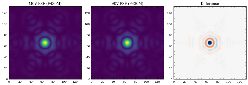
# Demonstrate the color difference of the PSF for different spectral types, same magnitude
sp_M0V = pynrc.stellar_spectrum('M0V', 10, 'vegamag', nrc.bandpass)
sp_A0V = pynrc.stellar_spectrum('A0V', 10, 'vegamag', nrc.bandpass)

# Generate oversampled PSFs (counts/sec)
hdul_M0V = nrc.calc_psf_from_coeff(sp=sp_M0V, return_oversample=True)
hdul_A0V = nrc.calc_psf_from_coeff(sp=sp_A0V, return_oversample=True)

psf_M0V = hdul_M0V[0].data
psf_A0V = hdul_A0V[0].data

fig, axes = plt.subplots(1,3, figsize=(12,4))

axes[0].imshow(psf_M0V**0.5)
axes[0].set_title('M0V PSF ({})'.format(nrc.filter))
axes[1].imshow(psf_A0V**0.5)
axes[1].set_title('A0V PSF ({})'.format(nrc.filter))

diff = psf_M0V - psf_A0V

minmax = np.abs(diff).max() / 2
axes[2].imshow(diff, cmap='RdBu', vmin=-minmax, vmax=minmax)
axes[2].set_title('Difference')

fig.tight_layout()
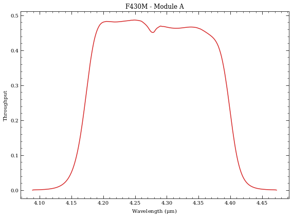
Bandpass information is stored in the bandpass attribute and can be plotted with the convenience function plot_bandpass().
[8]:
fig, ax = plt.subplots(1,1)
nrc.plot_bandpass(ax=ax, color='C3')

fig.tight_layout()
1. Saturation Limits
One of the most basic functions is to determine the saturation limit of a CDS observation, so let’s try this for the current filter selection. Generally, saturation is considered to be 80% of the full well, but can go as high as 95%.
[9]:
# Turn off those pesky informational texts
pynrc.setup_logging('WARN', verbose=False)

# Configure the observation for CDS frames (ngroup=2)
# Print out frame and ramp information using verbose=True
nrc.update_detectors(ngroup=2, verbose=True)
New Ramp Settings
  read_mode  :    RAPID
  nf         :        1
  nd2        :        0
  ngroup     :        2
  nint       :        1
New Detector Settings
  wind_mode  :     FULL
  xpix       :     2048
  ypix       :     2048
  x0         :        0
  y0         :        0
New Ramp Times
  t_group    :   10.737
  t_frame    :   10.737
  t_int      :   21.474
  t_int_tot1 :   21.474
  t_int_tot2 :    0.000
  t_exp      :   21.474
  t_acq      :   21.479
The sat_limits() function returns a dictionary of results. There’s the option in include a Pysynphot spectrum, but if None is specificed then it defaults to a G2V star.
[10]:
# Set verbose=True to print results in a user-friendly manner
sat_lims = nrc.sat_limits(verbose=True)

# Dictionary information
print("\nDictionary Info:", sat_lims)
F430M_ModA Saturation Limit assuming G2V source (point source): 12.24 vegamag
F430M_ModA Saturation Limit assuming G2V source (extended): 8.53 vegamag/arcsec^2

Dictionary Info: ({'satlim': 12.238364536563166, 'units': 'vegamag', 'bp_lim': 'F430M_ModA', 'Spectrum': 'G2V'}, {'satlim': 8.533744742439737, 'units': 'vegamag/arcsec^2', 'bp_lim': 'F430M_ModA', 'Spectrum': 'G2V'})
By default, the function sat_limits() uses a G2V stellar spectrum, but any arbritrary spectrum can be passed via the sp keyword. In addition, using the bp_lim keyword, you can use spectral information to determine the brightness in some other bandpass that saturates the source within the NIRCam filter.
[11]:
# Spectrum of an M0V star (not normalized)
sp_M0V = pynrc.stellar_spectrum('M0V')
# 2MASS Ks Bandpass
bp_k = pynrc.bp_2mass('K')

sat_lims = nrc.sat_limits(sp=sp_M0V, bp_lim=bp_k, verbose=True)
Ks-Band Saturation Limit for F430M_ModA assuming M0V source (point source): 12.31 vegamag
Ks-Band Saturation Limit for F430M_ModA assuming M0V source (extended): 8.61 vegamag/arcsec^2
Now, let’s get the same saturation limit assuming a 128x128 detector subarray (faster frame rate).
[12]:
nrc.update_detectors(wind_mode='WINDOW', xpix=128, ypix=128)
sat_lims = nrc.sat_limits(sp=sp_M0V, bp_lim=bp_k, verbose=True)
Ks-Band Saturation Limit for F430M_ModA assuming M0V source (point source): 7.89 vegamag
Ks-Band Saturation Limit for F430M_ModA assuming M0V source (extended): 4.18 vegamag/arcsec^2
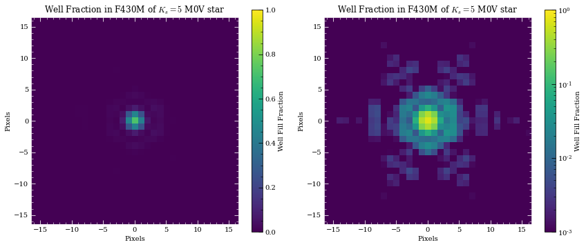
You can also use the saturation_levels() function to generate an image of a point source indicating the fractional well fill level.
[13]:
# Spectum of A0V star with Ks = 8 mag
sp = pynrc.stellar_spectrum('M0V', 8, 'vegamag', bp_k)
sat_levels = nrc.saturation_levels(sp, full_size=False, ngroup=nrc.det_info['ngroup'])

print('Max Well Fraction: {:.2f}'.format(sat_levels.max()))
Max Well Fraction: 0.72
[14]:
# Plot the well fill levels for each pixel
fig, axes = plt.subplots(1,2, figsize=(12,5))

for i,ax in enumerate(axes):
    extent = 0.5 * nrc.psf_info['fov_pix'] * np.array([-1,1,-1,1])
    if i==0:
        cax = ax.imshow(sat_levels, extent=extent, vmin=0, vmax=1)
    else:
        norm = matplotlib.colors.LogNorm(vmin=0.001, vmax=1)
        cax = ax.imshow(sat_levels, extent=extent, norm=norm)
    ax.set_xlabel('Pixels')
    ax.set_ylabel('Pixels')
    ax.set_title('Well Fraction in {} of $K_s = 5$ M0V star'.format(nrc.filter))

    cbar = fig.colorbar(cax, ax=ax)
    cbar.set_label('Well Fill Fraction')

    ax.tick_params(axis='both', color='white', which='both')
    for k in ax.spines.keys():
        ax.spines[k].set_color('white')

fig.tight_layout()
Information for slitless grism observations show wavelength-dependent results.
[15]:
nrc = pynrc.NIRCam(filter='F444W', pupil_mask='GRISM0', ngroup=2, wind_mode='STRIPE', ypix=128)
sat_lims = nrc.sat_limits(sp=sp_M0V, bp_lim=bp_k, verbose=True)
Ks-Band Saturation Limit for F444W_ModA_GRISMR assuming M0V source:
   Wave   Sat Limit (vegamag)
--------- -------------------
     3.90                4.79
     4.00                4.78
     4.10                4.67
     4.20                4.58
     4.30                4.43
     4.40                4.09
     4.50                3.91
     4.60                3.75
     4.70                3.57
     4.80                3.39
     4.90                3.17
     5.00                2.55
2. Sensitivity Limits
Similarly, we can determine sensitivity limits of point sources (and extended sources) for the defined instrument configuration. By default, the sensitivity() function uses a flat spectrum. In this case, let’s find the sensitivities NIRCam can reach in a single ~1000sec integration with the F430M filter. Noise values will depend on the exact MULTIACCUM settings.
[16]:
nrc = pynrc.NIRCam(filter='F430M')
nrc.update_detectors(read_mode='MEDIUM8', ngroup=10)

# The multiaccum_times attribute describes the various timing information
print(nrc.multiaccum_times)
[webbpsf_ext.imreg_tools:INFO] Recentered oversampled PSF (0.028, -0.017) pixels using Gaussian Fit algorithm.
{'t_frame': 10.73677, 't_group': 107.3677, 't_int': 1052.20346, 't_exp': 1052.20346, 't_acq': 1052.2087, 't_int_tot1': 1052.20346, 't_int_tot2': 0.0}
[17]:
sens = nrc.sensitivity(nsig=5, units='vegamag', verbose=True)
Point Source Sensitivity (5-sigma): 23.38 vegamag
Surface Brightness Sensitivity (5-sigma): 21.25 vegamag/arcsec^2
The sensitivity function also includes a keyword forwardSNR, which allows the user to pass a normalized spectrum and estimate the SNR For some extraction aperture.
[18]:
sp = pynrc.stellar_spectrum('M0V', 20, 'vegamag', nrc.bandpass)
snr = nrc.sensitivity(sp=sp, forwardSNR=True, units='vegamag', verbose=True)
Point Source SNR (20.00 vegamag): 79.06 sigma
Surface Brightness SNR (20.00 vegamag/arcsec^2): 14.93 sigma
3. Ramp Optimization
Armed with these two basic functions, we can attempt to determine the best instrument settings to optimize for SNR and efficiency. In these types of optimizations, we must consider observational constraints such as saturation levels, SNR requirements, and limits on acquisition time.
Note: The reported acquisition times do not include obsevatory and instrument-level overheads, such as slew times, filter changes, script compilations, etc. It only includes detector readout times (including reset frames and Fast Row Resets).
For instance, we want to observe an M-Dwarf (K=18 mag) in the F430M filter. What is the most efficient configuration to obtain an SNR of 100?
[19]:
# Setup observation
nrc = pynrc.NIRCam(filter='F430M', wind_mode='WINDOW', xpix=160, ypix=160)

# Spectrum of an M2V star
bp_k = pynrc.bp_2mass('K')
sp_M0V = pynrc.stellar_spectrum('M0V', 18, 'vegamag', bp_k)
[webbpsf_ext.imreg_tools:INFO] Recentered oversampled PSF (0.028, -0.017) pixels using Gaussian Fit algorithm.
[20]:
# Run optimizer. Result is a sorted by efficiency.
tbl = nrc.ramp_optimize(sp_M0V, snr_goal=100, ng_min=5, nint_min=10, verbose=True)
BRIGHT1
BRIGHT2
DEEP2
DEEP8
MEDIUM2
MEDIUM8
RAPID
SHALLOW2
SHALLOW4
 Pattern   NGRP NINT   t_int     t_exp     t_acq     SNR      Well     eff
---------- ---- ---- --------- --------- --------- -------- -------- --------
DEEP8         5   10     24.52    245.20    248.04    115.4    0.005    7.325
MEDIUM8       7   11     18.95    208.42    211.54    100.8    0.004    6.932
MEDIUM8       7   12     18.95    227.37    230.78    105.3    0.004    6.932
MEDIUM2       9   10     22.85    228.48    231.32    101.5    0.005    6.673
MEDIUM2       9   11     22.85    251.33    254.46    106.5    0.005    6.673
SHALLOW4     10   18     13.65    245.76    250.87    100.1    0.003    6.322
SHALLOW4     10   19     13.65    259.41    264.81    102.9    0.003    6.322
DEEP2         5   11     22.85    251.33    254.46     99.0    0.005    6.206
DEEP2         5   12     22.85    274.18    277.59    103.4    0.005    6.206
SHALLOW2     10   22     13.10    288.11    294.36     98.6    0.003    5.749
...         ...  ...       ...       ...       ...      ...      ...      ...
RAPID        10  632      2.79   1761.00   1940.37    101.3    0.001    2.298
RAPID        10  633      2.79   1763.79   1943.44    101.3    0.001    2.298
RAPID        10  634      2.79   1766.58   1946.51    101.4    0.001    2.298
RAPID        10  635      2.79   1769.36   1949.58    101.5    0.001    2.298
RAPID        10  636      2.79   1772.15   1952.65    101.6    0.001    2.298
RAPID        10  637      2.79   1774.94   1955.72    101.7    0.001    2.298
RAPID        10  638      2.79   1777.72   1958.79    101.7    0.001    2.298
RAPID        10  639      2.79   1780.51   1961.86    101.8    0.001    2.298
RAPID        10  640      2.79   1783.30   1964.93    101.9    0.001    2.298
RAPID        10  641      2.79   1786.08   1968.00    102.0    0.001    2.298
RAPID        10  642      2.79   1788.87   1971.07    102.1    0.001    2.298
Length = 55 rows
For a slightly more complicated scenario, consider an additional foreground source. In this scenario, the F0V star will saturate much more quickly compared to the fainter M2V, so it limits which ramp settings we may want to use (assuming we want unsaturated frames, which isn’t always necessarily true).
[21]:
sp_F0V = pynrc.stellar_spectrum('F0V', 10, 'vegamag', bp_k)
tbl = nrc.ramp_optimize(sp_M0V, sp_bright=sp_F0V, snr_goal=100, ng_min=5, nint_min=10,
                        well_frac_max=0.9, verbose=True)
BRIGHT1
BRIGHT2
DEEP2
DEEP8
MEDIUM2
MEDIUM8
RAPID
SHALLOW2
SHALLOW4
 Pattern   NGRP NINT   t_int     t_exp     t_acq     SNR      Well     eff
---------- ---- ---- --------- --------- --------- -------- -------- --------
RAPID        10  616      2.79   1716.42   1891.24    100.0    0.827    2.298
RAPID        10  617      2.79   1719.21   1894.31    100.1    0.827    2.298
RAPID        10  618      2.79   1722.00   1897.38    100.1    0.827    2.298
RAPID        10  619      2.79   1724.78   1900.45    100.2    0.827    2.298
RAPID        10  620      2.79   1727.57   1903.52    100.3    0.827    2.298
RAPID        10  621      2.79   1730.35   1906.59    100.4    0.827    2.298
RAPID        10  622      2.79   1733.14   1909.66    100.5    0.827    2.298
RAPID        10  623      2.79   1735.93   1912.73    100.5    0.827    2.298
RAPID        10  624      2.79   1738.71   1915.80    100.6    0.827    2.298
RAPID        10  625      2.79   1741.50   1918.88    100.7    0.827    2.298
...         ...  ...       ...       ...       ...      ...      ...      ...
BRIGHT1       5 1188      2.51   2979.22   3316.37    101.6    0.744    1.764
BRIGHT1       5 1189      2.51   2981.73   3319.16    101.6    0.744    1.764
BRIGHT1       5 1190      2.51   2984.23   3321.96    101.7    0.744    1.764
BRIGHT1       5 1191      2.51   2986.74   3324.75    101.7    0.744    1.764
BRIGHT1       5 1192      2.51   2989.25   3327.54    101.8    0.744    1.764
BRIGHT1       5 1193      2.51   2991.76   3330.33    101.8    0.744    1.764
BRIGHT1       5 1194      2.51   2994.27   3333.12    101.9    0.744    1.764
BRIGHT1       5 1195      2.51   2996.77   3335.91    101.9    0.744    1.764
BRIGHT1       5 1196      2.51   2999.28   3338.71    101.9    0.744    1.764
BRIGHT1       5 1197      2.51   3001.79   3341.50    102.0    0.744    1.764
BRIGHT1       5 1198      2.51   3004.30   3344.29    102.0    0.744    1.764
Length = 105 rows
If there are no objections to saturating the bright source, then we can set the well_frac_max parameter to something like 5 times the hard saturation limit. This allows for much more efficient exposure settings.
[22]:
tbl = nrc.ramp_optimize(sp_M0V, sp_bright=sp_F0V, snr_goal=100, ng_min=5, nint_min=10,
                        well_frac_max=5, verbose=True)
BRIGHT1
BRIGHT2
DEEP2
DEEP8
MEDIUM2
MEDIUM8
RAPID
SHALLOW2
SHALLOW4
 Pattern   NGRP NINT   t_int     t_exp     t_acq     SNR      Well     eff
---------- ---- ---- --------- --------- --------- -------- -------- --------
MEDIUM8       6   14     16.16    226.26    230.23     99.9    4.795    6.582
MEDIUM8       6   15     16.16    242.42    246.67    103.4    4.795    6.582
SHALLOW4     10   18     13.65    245.76    250.87    100.1    4.051    6.322
SHALLOW4     10   19     13.65    259.41    264.81    102.9    4.051    6.322
MEDIUM8       5   21     13.37    280.87    286.83    103.7    3.969    6.123
SHALLOW2     10   22     13.10    288.11    294.36     98.6    3.886    5.749
SHALLOW2     10   23     13.10    301.21    307.74    100.9    3.886    5.749
SHALLOW2     10   24     13.10    314.31    321.12    103.0    3.886    5.749
MEDIUM2       6   22     14.49    318.76    325.01     99.0    4.299    5.493
MEDIUM2       6   23     14.49    333.25    339.78    101.3    4.299    5.493
...         ...  ...       ...       ...       ...      ...      ...      ...
RAPID        10  632      2.79   1761.00   1940.37    101.3    0.827    2.298
RAPID        10  633      2.79   1763.79   1943.44    101.3    0.827    2.298
RAPID        10  634      2.79   1766.58   1946.51    101.4    0.827    2.298
RAPID        10  635      2.79   1769.36   1949.58    101.5    0.827    2.298
RAPID        10  636      2.79   1772.15   1952.65    101.6    0.827    2.298
RAPID        10  637      2.79   1774.94   1955.72    101.7    0.827    2.298
RAPID        10  638      2.79   1777.72   1958.79    101.7    0.827    2.298
RAPID        10  639      2.79   1780.51   1961.86    101.8    0.827    2.298
RAPID        10  640      2.79   1783.30   1964.93    101.9    0.827    2.298
RAPID        10  641      2.79   1786.08   1968.00    102.0    0.827    2.298
RAPID        10  642      2.79   1788.87   1971.07    102.1    0.827    2.298
Length = 54 rows
[ ]: